library("tidyverse")
library("sf")
raw_journey_data <- tribble(
~start.long, ~start.lat, ~end.long, ~end.lat, ~name,
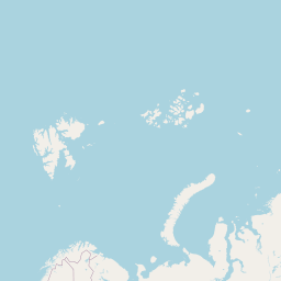
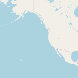
-0.118092, 51.509865, -119.698189, 34.420830, "London to Santa Barbara",
31.496773, 30.026300, 24.753574, 59.436962, "New Cairo to Tallinn",
126.633333, 45.75, 46.738586, 24.774265, "Harbin to Riyadh"
)
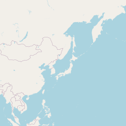
raw_journey_dataSurprisingly often I’m asked to help folks build maps which visualise the journeys between geographic locations, in the bad old days of early 2017 I would have used the geospheres package and sp.
That’s because the shortest distance between two points on a map is a great circle, and geospheres is capable of computing such things. Note that it’s these great circles that you see on flight information screens, their exact curvature depends on the projection of the map.
However, I’m now an sf convert and try to do everything within that package. In my original version of this blogpost I introduced my painfully inefficient way to compute these great circles with sf and asked folks in the R4DS Slack group run by Jesse Maegan if they had any suggested improvements, which I’ve now baked in below.
Typically my datasets are collections of journeys, here’s an example of what the data looks like (these are some of the journeys I took during the 3 years I worked for Wolfram Research):
I’ve split this post into two sections below:
- journeys_to_sf: A function for reliably converting journey data to an
sfobject that can be plotted withleafletandggplot2 - Creating
sffeatures fromdata.frames
journeys_to_sf
Here’s my function for converting a data.frame containing journeys to a usable "sf" "data.frame" through the use of tidyeval:
journeys_to_sf <- function(journeys_data,
start_long = start.long,
start_lat = start.lat,
end_long = end.long,
end_lat = end.lat) {
quo_start_long <- enquo(start_long)
quo_start_lat <- enquo(start_lat)
quo_end_long <- enquo(end_long)
quo_end_lat <- enquo(end_lat)
journeys_data %>%
select(
!! quo_start_long,
!! quo_start_lat,
!! quo_end_long,
!! quo_end_lat
) %>%
transpose() %>%
map(~ matrix(flatten_dbl(.), nrow = 2, byrow = TRUE)) %>%
map(st_linestring) %>%
st_sfc(crs = 4326) %>%
st_sf(geometry = .) %>%
bind_cols(journeys_data) %>%
select(everything(), geometry)
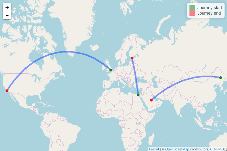
}This can very easily be inserted into a pipe chain for visualising with leaflet:
library("leaflet")
raw_journey_data %>%
  journeys_to_sf() %>%
  st_segmentize(units::set_units(100, km)) %>%
  leaflet() %>%
  addTiles() %>%
  addPolylines() %>%
  addCircleMarkers(
    lng = ~start.long,
    lat = ~start.lat,
    color = "green",
    opacity = 1,
    radius = 2
  ) %>%
  addCircleMarkers(
    lng = ~end.long,
    lat = ~end.lat,
    color = "red",
    opacity = 1,
    radius = 2
  ) %>%
  addLegend(
    colors = c(
      "green",
      "red"
    ),
    labels = c(
      "Journey start",
      "Journey end"
    )
  )

A quick note to say, leaflet is an awesome htmlwidget for building interactive maps. If you’ve never heard of htmlwidgets before, check out my blogpost; where’s the love for htmlwidgets?
Creating sf features from data.frame
The sf library allows R folks to work with GIS data using the very widely used Simple Features standard for working with 2D geometries. All sf objects are constructed from a combination of 17 unique “simple features”, which are usefully summarised here.
Originally my blogpost used a quite inefficient method for converting data.frame to sf. Thankfully I’m a member of the excellent R4DS Slack group and I got great advice from Jesse Sadler and Kent Johnson. Here’s my old horrible method of doing things:
start_locs <- raw_journey_data %>%
  select(
    start.long,
    start.lat
  ) %>%
  setNames(c("long", "lat")) %>%
  mutate(journey_id = row_number())

end_locs <- raw_journey_data %>%
  select(
    end.long,
    end.lat
  ) %>%
  setNames(c("long", "lat")) %>%
  mutate(journey_id = row_number())

journey_data_linestrings <- start_locs %>%
  bind_rows(end_locs) %>%
  st_as_sf(coords = c("long", "lat")) %>%
  group_by(journey_id) %>%
  arrange(journey_id) %>%
  summarise() %>%
  st_cast("LINESTRING")

journey_data_linestrings <- st_set_crs(journey_data_linestrings, st_crs(4326))

journey_data <- raw_journey_data
st_geometry(journey_data) <- st_geometry(journey_data_linestrings)
journey_data
Simple feature collection with 3 features and 5 fields
Geometry type: LINESTRING
Dimension: XY
Bounding box: xmin: -119.6982 ymin: 24.77426 xmax: 126.6333 ymax: 59.43696
Geodetic CRS: WGS 84
# A tibble: 3 × 6
start.long start.lat end.long end.lat name geometry
<dbl> <dbl> <dbl> <dbl> <chr> <LINESTRING [°]>
1 -0.118 51.5 -120. 34.4 London to San… (-119.6982 34.42083, -0.…
2 31.5 30.0 24.8 59.4 New Cairo to … (24.75357 59.43696, 31.4…
3 127. 45.8 46.7 24.8 Harbin to Riy… (46.73859 24.77426, 126.…Let’s go through the stages required and re-write my method to be more purrr dependent:
- Create a list of
LINESTRINGs - Combine the list
LINESTRINGs into a collection ofsffeatures - Join this collection of
sffeatures with the original dataset
LINESTRINGs
We need LINESTRINGs for our great circles as these represent a “sequence of points connected by straight, non-self intersecting line pieces; one-dimensional geometry”. As with all simple features, LINESTRINGs are constructed from matrices:
st_linestring(matrix(1:6, 3))LINESTRING (1 4, 2 5, 3 6)Let’s extract the start and end coordinates from our raw_journeys_data and convert them to a list with purrr::transpose:
raw_journey_data %>%
  select(-name) %>%
  transpose()
[[1]]
[[1]]$start.long
[1] -0.118092
[[1]]$start.lat
[1] 51.50986
[[1]]$end.long
[1] -119.6982
[[1]]$end.lat
[1] 34.42083
[[2]]
[[2]]$start.long
[1] 31.49677
[[2]]$start.lat
[1] 30.0263
[[2]]$end.long
[1] 24.75357
[[2]]$end.lat
[1] 59.43696
[[3]]
[[3]]$start.long
[1] 126.6333
[[3]]$start.lat
[1] 45.75
[[3]]$end.long
[1] 46.73859
[[3]]$end.lat
[1] 24.77426These lists can easily be converted to matrices using map:
raw_journey_data %>%
  select(-name) %>%
  transpose() %>%
  map(~ matrix(flatten_dbl(.), nrow = 2, byrow = TRUE))
[[1]]
[,1] [,2]
[1,] -0.118092 51.50986
[2,] -119.698189 34.42083
[[2]]
[,1] [,2]
[1,] 31.49677 30.02630
[2,] 24.75357 59.43696
[[3]]
[,1] [,2]
[1,] 126.63333 45.75000
[2,] 46.73859 24.77426… and finally we can convert these to
list_of_linestrings <- raw_journey_data %>%
  select(-name) %>%
  transpose() %>%
  map(~ matrix(flatten_dbl(.), nrow = 2, byrow = TRUE)) %>%
  map(st_linestring)
list_of_linestrings
LINESTRING (-0.118092 51.50986, -119.6982 34.42083)LINESTRING (31.49677 30.0263, 24.75357 59.43696)LINESTRING (126.6333 45.75, 46.73859 24.77426)Collecting features
Eventually we will create an "sf" "data.frame" which contains our LINESTRINGs in the geometry column. We create a set of features for this column from our list of LINESTRINGs with the st_sfc function. Note that we need to specify a coordinate system, the most obvious choice is the WGS84 coordinate reference system, that’s why we specify crs = 4326:
list_of_linestrings %>%
  st_sfc(crs = 4326)
Geometry set for 3 features
Geometry type: LINESTRING
Dimension: XY
Bounding box: xmin: -119.6982 ymin: 24.77426 xmax: 126.6333 ymax: 59.43696
Geodetic CRS: WGS 84Now we have this set of features we create a collection of them in a "sf" "data.frame" with st_sf:
collection_sf <- list_of_linestrings %>%
  st_sfc(crs = 4326) %>%
  st_sf(geometry = .)
collection_sf
Simple feature collection with 3 features and 0 fields
Geometry type: LINESTRING
Dimension: XY
Bounding box: xmin: -119.6982 ymin: 24.77426 xmax: 126.6333 ymax: 59.43696
Geodetic CRS: WGS 84
geometry
1 LINESTRING (-0.118092 51.50...
2 LINESTRING (31.49677 30.026...
3 LINESTRING (126.6333 45.75,...Joining feature collections with data
As sf collections store all of the GIS data in a column it’s very easy to combine this object with our original data - we use dplyr::bind_columns
collection_sf %>%
  bind_cols(raw_journey_data)
Simple feature collection with 3 features and 5 fields
Geometry type: LINESTRING
Dimension: XY
Bounding box: xmin: -119.6982 ymin: 24.77426 xmax: 126.6333 ymax: 59.43696
Geodetic CRS: WGS 84
start.long start.lat end.long end.lat name
1 -0.118092 51.50986 -119.69819 34.42083 London to Santa Barbara
2 31.496773 30.02630 24.75357 59.43696 New Cairo to Tallinn
3 126.633333 45.75000 46.73859 24.77426 Harbin to Riyadh
geometry
1 LINESTRING (-0.118092 51.50...
2 LINESTRING (31.49677 30.026...
3 LINESTRING (126.6333 45.75,...We can now perform calculations on our dataset, for instance compute great circles with a resolution of 100km:
collection_sf %>%
  bind_cols(raw_journey_data) %>%
  st_segmentize(units::set_units(100, km)) %>%
  leaflet() %>%
  addTiles() %>%
addPolylines(label = ~name)Sadly, there’s no good solution for adding arrow heads to these great circles - they would be heavily distorted by the map projection and would look ugly. An alternative solution to showing where journeys start and end is to use different coloured circle markers:
collection_sf %>%
  bind_cols(raw_journey_data) %>%
  st_segmentize(units::set_units(100, km)) %>%
  leaflet() %>%
  addTiles() %>%
  addPolylines() %>%
  addCircleMarkers(
    lng = ~start.long,
    lat = ~start.lat,
    color = "green",
    opacity = 1,
    radius = 2
  ) %>%
  addCircleMarkers(
    lng = ~end.long,
    lat = ~end.lat,
    color = "red",
    opacity = 1,
    radius = 2
  ) %>%
  addLegend(
    colors = c(
      "green",
      "red"
    ),
    labels = c(
      "Journey start",
      "Journey end"
    )
)Reuse
Citation
BibTeX citation:
@online{hadley2018,
  author = {Charlie Hadley},
  title = {Great Circles with Sf and Leaflet},
  date = {2018-02-28},
  url = {https://visibledata.co.uk/posts/2018-02-28_great-circles-with-sf-and-leaflet},
  langid = {en}
}
For attribution, please cite this work as:
Charlie Hadley. 2018. “Great Circles with Sf and Leaflet.”
February 28, 2018. https://visibledata.co.uk/posts/2018-02-28_great-circles-with-sf-and-leaflet.